import statsmodels.api as sm
import pandas
from patsy import dmatrices21 StatsModel — Basic
StatsModels is a Python library for statistical modeling and econometrics. It provides classes and functions for estimating various statistical models, conducting statistical tests, and exploring data. StatsModels complements SciPy and provides a more comprehensive set of tools for statistical analysis.
Key features of StatsModels include:
- Linear regression models
- Generalized linear models
- Robust linear models
- Linear mixed effects models
- Time series analysis tools
- Nonparametric methods
- Visualization of statistical model results
In this notebook, we’ll explore basic usage of StatsModels for linear regression.
21.1 Data Download
For this example, we’ll use the Guerry dataset, a historical dataset collected by André-Michel Guerry in the 1830s. It contains data about crime, literacy, poverty, and other moral statistics for departments in France.
The dataset is accessible through StatsModels’ get_rdataset function, which imports datasets from R packages.
The Guerry dataset includes variables such as:
- Lottery: Per capita wager on Royal Lottery
- Literacy: Percent of military conscripts who can read and write
- Wealth: Tax on personal property
- Region: Geographic region (N, E, S, W, C for North, East, South, West, Central)
df = sm.datasets.get_rdataset("Guerry", "HistData").data
df.head()| dept | Region | Department | Crime_pers | Crime_prop | Literacy | Donations | Infants | Suicides | MainCity | ... | Crime_parents | Infanticide | Donation_clergy | Lottery | Desertion | Instruction | Prostitutes | Distance | Area | Pop1831 | |
|---|---|---|---|---|---|---|---|---|---|---|---|---|---|---|---|---|---|---|---|---|---|
| 0 | 1 | E | Ain | 28870 | 15890 | 37 | 5098 | 33120 | 35039 | 2:Med | ... | 71 | 60 | 69 | 41 | 55 | 46 | 13 | 218.372 | 5762 | 346.03 |
| 1 | 2 | N | Aisne | 26226 | 5521 | 51 | 8901 | 14572 | 12831 | 2:Med | ... | 4 | 82 | 36 | 38 | 82 | 24 | 327 | 65.945 | 7369 | 513.00 |
| 2 | 3 | C | Allier | 26747 | 7925 | 13 | 10973 | 17044 | 114121 | 2:Med | ... | 46 | 42 | 76 | 66 | 16 | 85 | 34 | 161.927 | 7340 | 298.26 |
| 3 | 4 | E | Basses-Alpes | 12935 | 7289 | 46 | 2733 | 23018 | 14238 | 1:Sm | ... | 70 | 12 | 37 | 80 | 32 | 29 | 2 | 351.399 | 6925 | 155.90 |
| 4 | 5 | E | Hautes-Alpes | 17488 | 8174 | 69 | 6962 | 23076 | 16171 | 1:Sm | ... | 22 | 23 | 64 | 79 | 35 | 7 | 1 | 320.280 | 5549 | 129.10 |
5 rows × 23 columns
vars = ['Department', 'Lottery', 'Literacy', 'Wealth', 'Region']
df = df[vars]
df[-5:]| Department | Lottery | Literacy | Wealth | Region | |
|---|---|---|---|---|---|
| 81 | Vienne | 40 | 25 | 68 | W |
| 82 | Haute-Vienne | 55 | 13 | 67 | C |
| 83 | Vosges | 14 | 62 | 82 | E |
| 84 | Yonne | 51 | 47 | 30 | C |
| 85 | Corse | 83 | 49 | 37 | NaN |
21.2 Preprocess
Before fitting our model, we need to ensure the data is clean. The following step drops any rows with missing values (NaN) to ensure our model receives complete data points only.
df = df.dropna()
df.head()| Department | Lottery | Literacy | Wealth | Region | |
|---|---|---|---|---|---|
| 0 | Ain | 41 | 37 | 73 | E |
| 1 | Aisne | 38 | 51 | 22 | N |
| 2 | Allier | 66 | 13 | 61 | C |
| 3 | Basses-Alpes | 80 | 46 | 76 | E |
| 4 | Hautes-Alpes | 79 | 69 | 83 | E |
21.3 Formula Interface and Design Matrices
StatsModels supports a formula interface similar to R, using the Patsy library to specify models. This approach allows for a more intuitive specification of regression models.
The dmatrices function creates design matrices from a formula string:
- Left side of
~specifies the dependent variable (y) - Right side specifies the independent variables (X)
- Categorical variables (like Region) are automatically converted to dummy variables
- An intercept term is included by default
In our model, we’re trying to predict Lottery (per capita lottery wagers) based on Literacy, Wealth, and Region.
y, X = dmatrices('Lottery ~ Literacy + Wealth + Region', data=df, return_type='dataframe')y[:3]| Lottery | |
|---|---|
| 0 | 41.0 |
| 1 | 38.0 |
| 2 | 66.0 |
X[:3]| Intercept | Region[T.E] | Region[T.N] | Region[T.S] | Region[T.W] | Literacy | Wealth | |
|---|---|---|---|---|---|---|---|
| 0 | 1.0 | 1.0 | 0.0 | 0.0 | 0.0 | 37.0 | 73.0 |
| 1 | 1.0 | 0.0 | 1.0 | 0.0 | 0.0 | 51.0 | 22.0 |
| 2 | 1.0 | 0.0 | 0.0 | 0.0 | 0.0 | 13.0 | 61.0 |
21.4 Model Fitting and Summary
Now that we have our design matrices, we can fit an Ordinary Least Squares (OLS) regression model. The process involves two steps:
- Create a model specification using
sm.OLS() - Fit the model to the data using
.fit()
The resulting model object contains parameter estimates and various statistics that help evaluate the model’s performance.
mod = sm.OLS(y, X)    # Describe model
mod
<statsmodels.regression.linear_model.OLS at 0x169d07c20>res = mod.fit() # Fit model
res<statsmodels.regression.linear_model.RegressionResultsWrapper at 0x169dd2ae0>21.4.1 Summary Results
The summary output provides comprehensive statistics about the model:
- Coefficient estimates: The estimated effect of each predictor on the response variable
- Standard errors: Measure of the statistical precision of the coefficient estimates
- t-statistics and p-values: Used to test the null hypothesis that a coefficient is zero
- R-squared: Proportion of variance in the dependent variable explained by the model
- Adjusted R-squared: R-squared adjusted for the number of predictors
- F-statistic: Tests the overall significance of the regression
- AIC/BIC: Information criteria for model comparison
StatsModels provides two summary methods: summary() and summary2(), each with slightly different presentation formats.
res.summary()| Dep. Variable: | Lottery | R-squared: | 0.338 |
| Model: | OLS | Adj. R-squared: | 0.287 |
| Method: | Least Squares | F-statistic: | 6.636 |
| Date: | Fri, 18 Apr 2025 | Prob (F-statistic): | 1.07e-05 |
| Time: | 21:01:25 | Log-Likelihood: | -375.30 |
| No. Observations: | 85 | AIC: | 764.6 |
| Df Residuals: | 78 | BIC: | 781.7 |
| Df Model: | 6 | ||
| Covariance Type: | nonrobust |
| coef | std err | t | P>|t| | [0.025 | 0.975] | |
| Intercept | 38.6517 | 9.456 | 4.087 | 0.000 | 19.826 | 57.478 |
| Region[T.E] | -15.4278 | 9.727 | -1.586 | 0.117 | -34.793 | 3.938 |
| Region[T.N] | -10.0170 | 9.260 | -1.082 | 0.283 | -28.453 | 8.419 |
| Region[T.S] | -4.5483 | 7.279 | -0.625 | 0.534 | -19.039 | 9.943 |
| Region[T.W] | -10.0913 | 7.196 | -1.402 | 0.165 | -24.418 | 4.235 |
| Literacy | -0.1858 | 0.210 | -0.886 | 0.378 | -0.603 | 0.232 |
| Wealth | 0.4515 | 0.103 | 4.390 | 0.000 | 0.247 | 0.656 |
| Omnibus: | 3.049 | Durbin-Watson: | 1.785 |
| Prob(Omnibus): | 0.218 | Jarque-Bera (JB): | 2.694 |
| Skew: | -0.340 | Prob(JB): | 0.260 |
| Kurtosis: | 2.454 | Cond. No. | 371. |
Notes:
[1] Standard Errors assume that the covariance matrix of the errors is correctly specified.
res.summary2()| Model: | OLS | Adj. R-squared: | 0.287 |
| Dependent Variable: | Lottery | AIC: | 764.5986 |
| Date: | 2025-04-18 21:01 | BIC: | 781.6971 |
| No. Observations: | 85 | Log-Likelihood: | -375.30 |
| Df Model: | 6 | F-statistic: | 6.636 |
| Df Residuals: | 78 | Prob (F-statistic): | 1.07e-05 |
| R-squared: | 0.338 | Scale: | 436.43 |
| Coef. | Std.Err. | t | P>|t| | [0.025 | 0.975] | |
| Intercept | 38.6517 | 9.4563 | 4.0874 | 0.0001 | 19.8255 | 57.4778 |
| Region[T.E] | -15.4278 | 9.7273 | -1.5860 | 0.1168 | -34.7934 | 3.9378 |
| Region[T.N] | -10.0170 | 9.2603 | -1.0817 | 0.2827 | -28.4528 | 8.4188 |
| Region[T.S] | -4.5483 | 7.2789 | -0.6249 | 0.5339 | -19.0394 | 9.9429 |
| Region[T.W] | -10.0913 | 7.1961 | -1.4023 | 0.1648 | -24.4176 | 4.2351 |
| Literacy | -0.1858 | 0.2098 | -0.8857 | 0.3785 | -0.6035 | 0.2319 |
| Wealth | 0.4515 | 0.1028 | 4.3899 | 0.0000 | 0.2467 | 0.6562 |
| Omnibus: | 3.049 | Durbin-Watson: | 1.785 |
| Prob(Omnibus): | 0.218 | Jarque-Bera (JB): | 2.694 |
| Skew: | -0.340 | Prob(JB): | 0.260 |
| Kurtosis: | 2.454 | Condition No.: | 371 |
Notes:
[1] Standard Errors assume that the covariance matrix of the errors is correctly specified.
21.4.2 Extracting Model Parameters
After fitting the model, we can extract specific statistics for further analysis or visualization:
params: Coefficient estimates for each predictorrsquared: R-squared value (goodness of fit)bse: Standard errors of the coefficient estimatespvalues: p-values for the t-tests of the coefficientsconf_int(): Confidence intervals for the coefficients
These attributes allow us to easily access specific pieces of information from the model results.
res.paramsIntercept 38.651655
Region[T.E] -15.427785
Region[T.N] -10.016961
Region[T.S] -4.548257
Region[T.W] -10.091276
Literacy -0.185819
Wealth 0.451475
dtype: float64res.rsquarednp.float64(0.337950869192882)21.5 Model Interpretation
When interpreting the regression results, consider the following:
Coefficients: Each coefficient represents the average change in the dependent variable (Lottery) for a one-unit increase in the predictor, holding other predictors constant.
Statistical significance: Look at p-values to determine if the relationship is statistically significant (typically p < 0.05).
Effect size: Consider not just significance but the magnitude of coefficients.
Model fit: The R-squared value indicates how much of the variation in lottery wagers is explained by our model.
Categorical variables: For Region variables (e.g., Region[T.E]), the coefficient represents the difference in the response compared to the reference category (in this case, Region C - Central).
In this model, we’re investigating whether literacy rates, wealth, and geographic region can predict lottery participation rates in 19th century France.
21.6 Plots
sm.graphics.plot_partregress('Lottery', 'Wealth', ['Region', 'Literacy'],
                             data=df, obs_labels=False)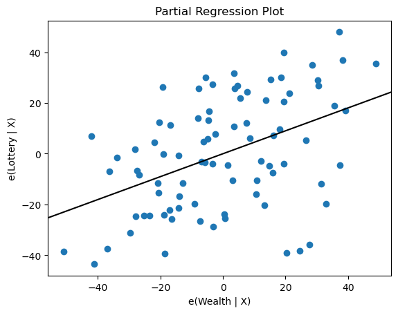

21.7 Additional Analysis
For a more complete analysis, you might want to explore:
- Residual analysis: Check if the residuals follow a normal distribution and have constant variance
- Outlier detection: Identify influential observations that might be driving the results
- Multicollinearity: Assess if predictors are highly correlated, which can affect coefficient estimates
- Model comparison: Compare different model specifications to find the best fit
- Predictions: Use the model to make predictions on new data
StatsModels provides tools for all these additional analyses.